Using Machine Learning to predict the S&P 500 price change, using the dark pool indicators Dix and Gex

This is the first version of an analysis I wanted to perform with the main purpose of learning. By this reason I have limited the number of input data and operations to the minimum.

To do something different I will be looking for correlations between the two main dark pool indexes: DIX and GEX Indexes. For more information about these indexes: https://joapen.com/blog/2019/10/15/dix-and-gex-indicators/

If you are interested to use this code to earn some dollars, this is not a good idea, maybe in future the new versions are more accurate and they can be used for that purpose. You always can take this code and make it better. It’s not difficult, I promise you.

Note 1 : To see the complete set of code and the results you need a Kaggle user.

Note 2: I’m not a professional developer, so you will see code that is written in a weird way, my apologizes.

My purpose of this post is to review some main aspects of the code.

1.- Import data and add some content

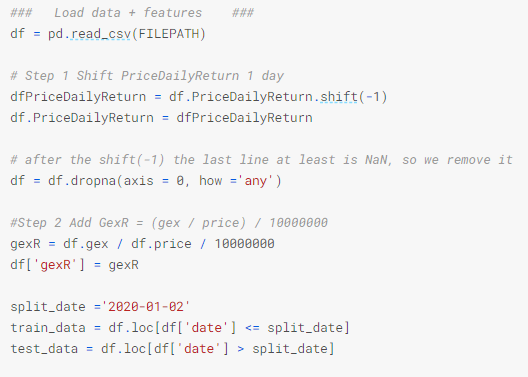
I have exported the data from squeezemetrics and after that I have created some new columns: PriceDailyReturn, DixDailyReturn and GexDailyReturn.

I started the analysis focusing on “price” as target value I wanted to predict, but I have found that “PriceDailyReturn” is a better target, mainly because it does inherit the previous days errors.

I have shifted the “PriceDailyReturn” so I am predicting the future, not the present.

I have added a new column to the data frame called gexR, I found it as something used by others and I wanted to see if it was useful or not.

I have split the data in training and test using 2/January/2020. This result in 2182 entries for training and 332 for testing.

2.- Exploratory Data Analysis (EDA)

I have created several charts to explore the data and try to see how it looks like. Some of the charts are used to see if there is any NaN value and the others just to see correlations and potential trends. For instance:

Another interesting one is the SPX price and the gexR representation:

3.- Feature Engineering

At this part of the data analysis I have not done anything. I still need to get more data and then, study each one of the features in deep.

4.- Train/test split of data

I have already split the data, so nothing here.

5.- Classification and model

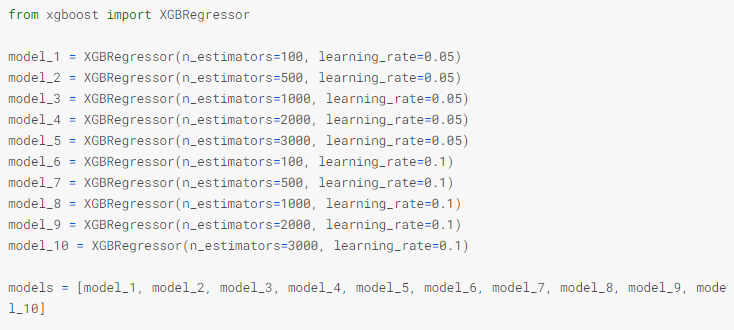
I have decided to use XGBoost library and a regressor as model.

I have learned that general, a small learning rate (and large number of estimators) will yield more accurate XGBoost models. This combination will also take the model longer to train since it does more iterations through the cycle.

As I do not know the right combination of parameters , I have done an initial review of them and I will pick up the more accurate.

Once defined, I’ve run each one of the models and check its mean absolute error (MAE):

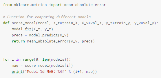
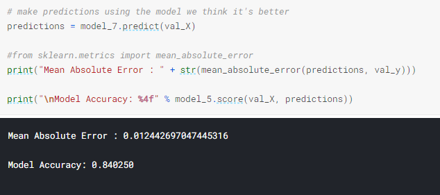
From model 7 to model 10 the median absolute error (MAE) is similar. So I use model 7 as the valid one right now.

6.- Let’s check the results

A basic chart with the actual data and the forecasted data:

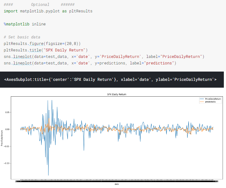
Visually, the behavior is fine when there are not so much changes, but this test data contains the big fall of March 2020, so there the predicted results are really bad (not a surprise with that few amount of parameters and data).

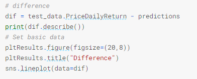
I have calculated the difference between the actuals and the prediction, and then I have plotted it:

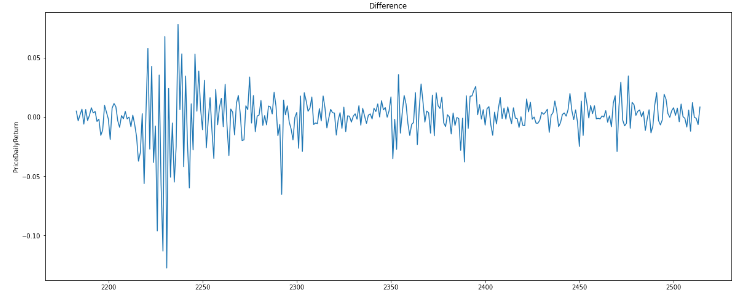
6.1.- performance of the prediction: TP, FP, TN, FN

I asked myself: how right or wrong is this prediction?

So to answer it I defined what are the true/false positives and the true/false negatives. I have defined a threshold of difference that I accept as valid, a type of accuracy that satisfies me.

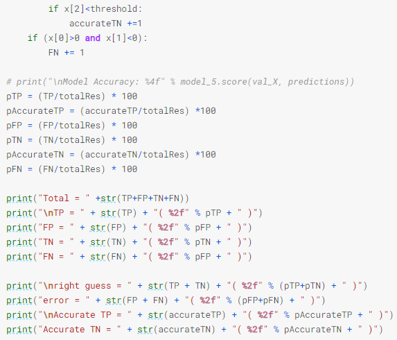
The results are:

Conclusion

A lot of learning doing this exercise, and I hope to have some time to improve the input data, the features analysis and the model selected.

If you have some suggestions or comments, please let me know, constructive feedback is more than welcome.