This post gather the analysis of data done with market breadth data, VIX, DIX and GEX. They are moved into a Long Short Term Memory (LSTM) neural network, that is a recurrent neural network.
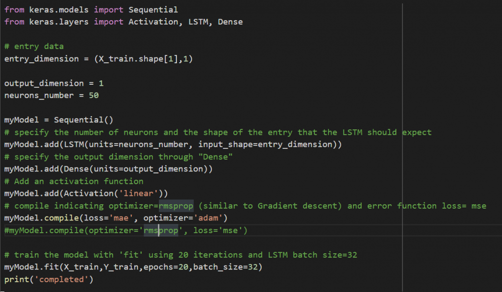
You can check the code and read how the whole thing is done.
Input data
The used features as input are:
Data ranges of input files (From -> To):
- Market breadth (1979-12-31 -> 2021-05-25 ).
- DIX and gex (2011-05-02 -> 2021-05-25).
- VIX (1990-01-02 -> 2021-05-25).
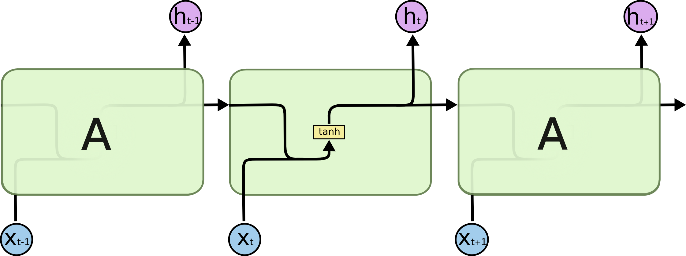
The LSTM neural network
This is the basic version of a recurrent neural network:
LSTM neural network simplified diagram:
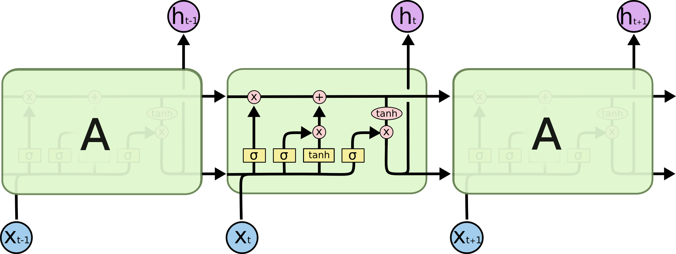
To understand the diagram in detail you can read this article. Some notes for my poor memory:
- The upper line with “X” and “+” symbols represents the cell state’s, which purpose is to decide what information to carry forward from the different observations.
- The left side of the input is composed by 2 steps: the input gate layer and the tanh layer. These layers work together to determine how to update the cell state.
- The right side of the LSTM determines the output for this observation. This step runs through both a sigmoid function and a hyperbolic tangent function.
More about forecasting, you can find on Joaquín’s Github this repository: https://github.com/JoaquinAmatRodrigo/skforecast , that contains a very useful notebook: https://github.com/JoaquinAmatRodrigo/skforecast/blob/master/notebooks/introduction_skforecast.ipynb
Optimizers used during this test
- Adam optimization is a stochastic gradient descent method that is based on adaptive estimation of first-order and second-order moments.
- SGD: Gradient descent (with momentum) optimizer.
- RMSprop: The gist of RMSprop is to 1) maintain a moving (discounted) average of the square of gradients; and 2) Divide the gradient by the root of this average.
One of the tests I have not performed is to define different parameters for the optimizers. There is a good bunch of alternatives you can play with, but as the initial results are not good, it does not makes sense to me to dig in. These ones are:
tf.keras.optimizers.Adam(
    learning_rate=0.001,
    beta_1=0.9,
    beta_2=0.999,
    epsilon=1e-07,
    amsgrad=False,
    name="Adam",
    **kwargs
)
tf.keras.optimizers.SGD(
    learning_rate=0.01, momentum=0.0, nesterov=False, name="SGD", **kwargs
)
tf.keras.optimizers.RMSprop(
    learning_rate=0.001,
    rho=0.9,
    momentum=0.0,
    epsilon=1e-07,
    centered=False,
    name="RMSprop",
    **kwargs
)
Basic correlation
Initially there is not a high correlation between SPX and other input features, but let’s see what happens, this is an experiment.

The challenges to me to build the neural network on Keras have been:
- Transform the matrix of 21 input parameters into a normalized matrix.
- Look for the more convenient optimizer.
- Understand the influence of the activation function.
- Work with matrix to adapt the visual representation of the results.
- Do the reverse transformation to visualize the prediction in the right amounts.
- I am using a recursive forecasting model so by definition I define a “time step”, that in my case is defined initially at 60, so it works on 60 rows of data and then it returns the 61 as result or prediction. This can be seen on the visual test where the first 60 values of the prediction are set to zero.
Visual result
This is the first result I obtained:
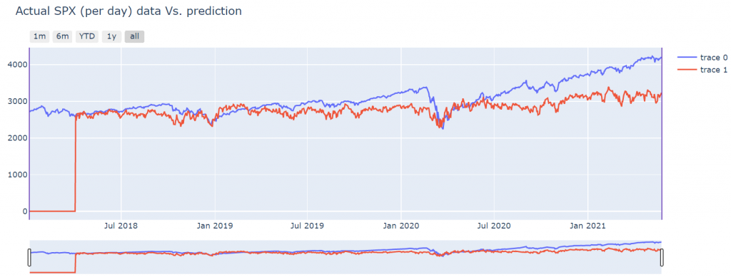
I have adjusted the relative result with an offset. That uses the first value of the prediction and the first actual value to define this offset.
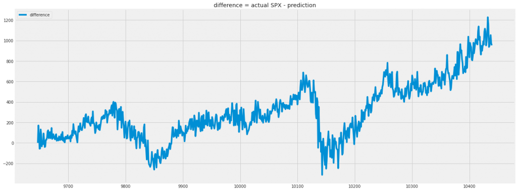
The initial results are not too bad, but the degradation of the results with respect the time makes the this result to be very poor as the difference between real and predicted number is bad:
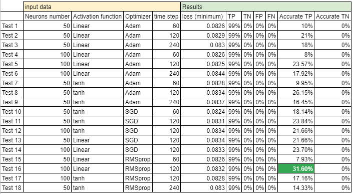
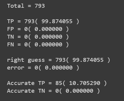
Results of the experiment
I have created a true positive, true negative, false positive and false negative table. I have defined 5 basic points of the SPX as threshold, below these 5 basic points of difference between actual value and predicted value the result is considered as accurate, above 5 basic points, it is considered as not accurate.
On this initial test only 10% of the tests are accurate.
The common parameters of all tests have been:
- Loss=mae
- epochs=20
- training_data = 9647
- test_data = 793
- Accuracy = 5 basic points of SPX
Table of results